Tutorial

Profiling a simple program

This tutorial explains how to profile a program with aprof and how to analyze the collected profiling data using aprof-plot.

A simple program

Suppose we want to analyze the performance of our implementation of a quick sort algorithm. For example, this can be our program code:

#include <stdlib.h>
#include <time.h>
#include <stdio.h>

int partition(int v[], int a, int b) {
	int pivot = a;
	for (;;) {
		while (a < b && v[a] <= v[pivot]) a++;
		while (v[b] > v[pivot]) b--;
		if (a >= b) break;
		int temp = v[a];
		v[a] = v[b];
		v[b] = temp;
	}
	if (v[b] != v[pivot]) {
		int temp = v[b];	
		v[b] = v[pivot];
		v[pivot] = temp;
	}
	return b;
}

void quick_sort_ric(int v[], int a, int b) {
	int m;
	if (a >= b) return;
	m = partition(v, a, b);
	quick_sort_ric(v, a, m-1);
	quick_sort_ric(v, m+1, b);
}

int main() {
    
	int v[1024*10];
	srand(time(0));
	int n = sizeof(v)/sizeof(int);
	int j = n, i = 0;

	for (j = 0; j < n; j += 100) {
	
		for (i = 0; i < j; i++)
			v[i] = rand() % (j+1);

		quick_sort_ric(v, 0, j-1);
	}
	
	printf("End\n");

	return 0;
}

The main function invokes our quick sort implementation different times. Each time the array is filled with some random numbers. In a real program probably our quick sort implementation would be called during the normal execution of our application and so we don't need to create an unrealistic main in order to profile our code. quick_sort_ric and partition are textbook implementations and therefore they are not very optimized (the first element of the array is chosen as pivot by partition).

We expect that:

• partition should be O(n)
• quick_sort_ric should be O( n * log(n) ) because the input is composed by random integers (average case performance).

Compiling the program

In order to profile our code we don't need any special compilation flag (e.g, -g or -pg). The only requirement is that our application binary should not be stripped out of the function symbols (by default GCC does not strip a binary). So, we can compile our example code in the usual way:

gcc -o quick_tutorial quick_tutorial.c

where quick_tutorial.c is a text file containing the previous example code.

Profiling

You can install aprof by following the Instructions for installing aprof. We can profile our program with the following command:

path-to-aprof/inst/bin/valgrind --tool=aprof ./quick_tutorial

The output should be somithing like this:

==28001== aprof-0.1.1, Input-sensitive Profiler - http://code.google.com/p/aprof/
==28001== by Emilio Coppa, Camil Demetrescu, Irene Finocchi
==28001== Using Valgrind-3.9.0.SVN and LibVEX; rerun with -h for copyright info
==28001== Command: ./quick_tutorial
==28001== 
End
==28001==

The first and last line of the output provide us the PID (28001) of the program execution. In the current working directory we should find a report called quick_tutorial_28001_0_4.aprof. This report is a text-file written following the aprof report file format.

Analyzing the profiling data

In order to analyze our report we can use aprof-plot, a Java tool for visualizing reports generated by aprof. You can install aprof-plot by following the Instructions for installing aprof-plot. You can run it by following the basic usage guide.

Open the report

Open the report in aprof-plot using the menu File > Open File... and search the report in your filesystem. This is what you should see:

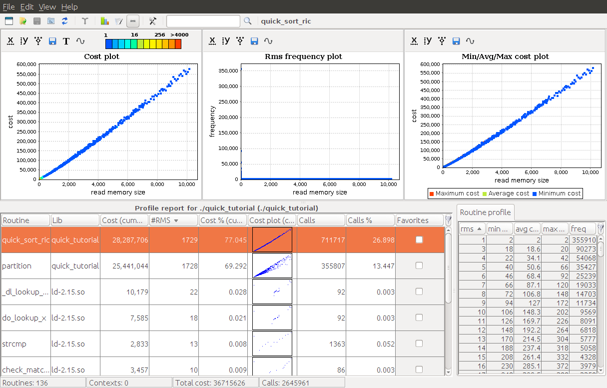
We can identify three main graphical components:

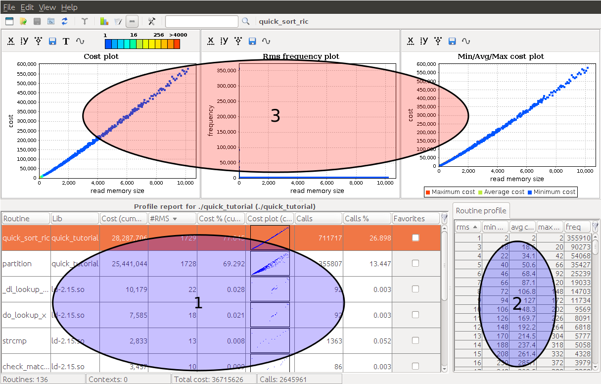
The first component is the routine table. This a list of all profiled routines of your program with several useful information (e.g., name, cumulative cost, number of collected RMS, etc.).

The second component is the routine profile. If you select a function in the routine table, then this component displays all the collected tuples (RMS value, min cost, max cost, frequency, etc.) for the chosen routine.

Finally, the third component displays several charts for the current selected routine.

In order to have a more detailed explanation of all aprof-plot components and features please see our aprof-prof manual.

Analyze our quick sort implementation

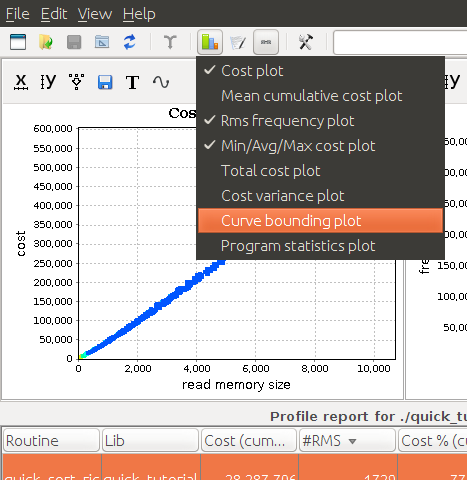
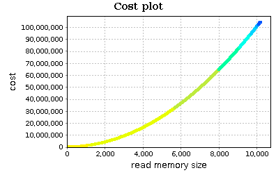
Let's focus on our quick sort implementation. Select quick_sort_ric function in the routine table and observe the cost plot chart (the first one):

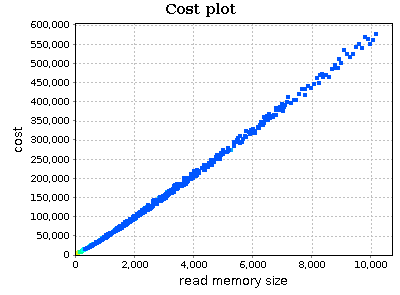
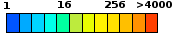
On x axis we have the RMS metric. This can be seen as an estimate of input sizes on which your function was executed. Instead, on y axis we find an execution cost metric (by default aprof counts the number of executed basic blocks). Points of the chart are colored based on their frequency (number of times your routine was executed on a specific RMS). The legend on the top specifies the frequency value of each color:

Select an area of the chart with your mouse in order to zoom in and better analyze points for small values of RMS:

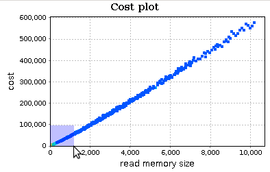
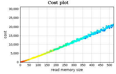
This chart reveals two things:

• the trend of quick_sort_ric does not appear to be quadratic; perhaps linear or n*log(n);
• quick_sort_ric is executed on small input sizes most of the times (the smaller is the RMS, the higher is the frequency): this is expected as quick sort is a divide-and-conquer sorting algorithm.

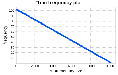
We can analyze in more detail our input workload using the RMS frequency plot (the second one; the chart is zoomed in):

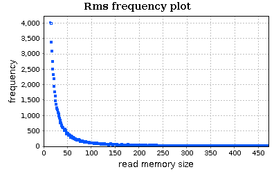
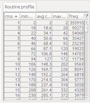
This chart confirms our observation on the frequency of input sizes. The routine profile, shown on the right, can be useful if we want to know the exact frequency (or cost) of each RMS value.

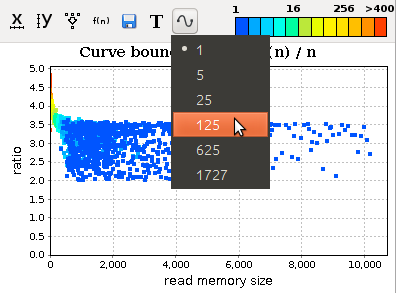
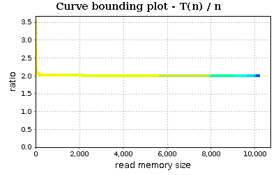
Now, enable the curve bounding plot:

By scrolling down the charts' area, you should see this new chart:

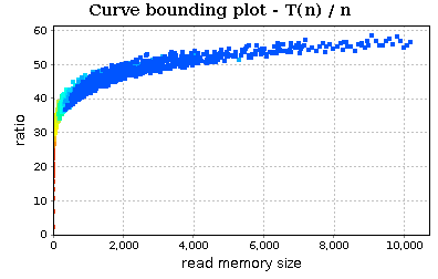
This chart allows us to simply apply the guess ratio rule. This is a simple method for evaluating the growth rate of a function by considering a guess function H(n) and analyzing the trend of ratio T(n)/H(n) (where T(n) is the function cost of our routine and n the RMS values). If T ∈ O(H), then the ratio will stabilize to a non-negative constant, while if T ∉ O(H) it (eventually) increases.

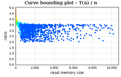
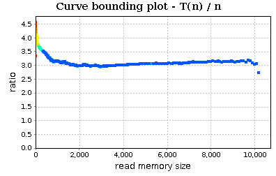
In the last screenshot, we observe that the trend of ratio T(n)/n (where T(n) is cost of our routine and n is the value of RMS) does not stabilize to a constant. Our next guess should be n * log(n):

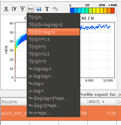
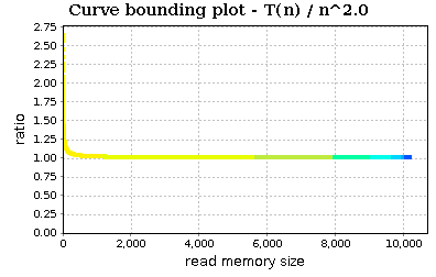
The trend stabilizes to a constant :) If we try with n^2:

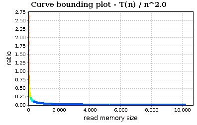
Zoom in:

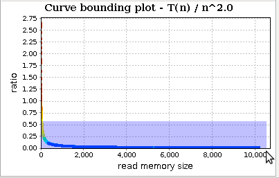
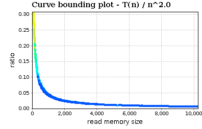
The trend slowly decreases. In conclusion, the visualized profiles seem to confirm that our implementation of quick sort (and in particular of quick_sort_ric) is bounded by O(n * log(n)).

Now, select in the routine table the partition function. Its curve bounding plot is:

The chart is a little bit chaotic. We can smooth the trend:

We can see that the trend (almost) stabilizes to a specific constant and therefore our partition routine can be assumed to be linear (at least on the tested workload).

A different workload

Our implementation of quick sort is efficient on a workload composed by random integers. But what happens if we change our workload? Maybe the workload of our application is unknown to us. We can see how the performance of our code changes if we sort a sorted array. For example, we can modify the main function in this way:

int main() {
    
	int v[1024*10];
	int n = sizeof(v)/sizeof(int);
	int j = n, i = 0;

	for (j = 0; j < n; j += 100) {
	
		for (i = 0; i < j; i++)
			v[i] = i;

		quick_sort_ric(v, 0, j-1);
	}
    
	printf("End\n");
    
	return 0;
}

If we profile the program and open the new report, we can see that quick_sort_ric has a clear quadratic trend:

This is the result of our pivot choice. Of course the trend of partition does not change: it remains linear but the trend is a lot neater:

In conclusion with aprof and aprof-plot we can profile our application, obtain clues about groth rates of our routines and possibly find some asymptotic bottlenecks. Moreover, we can understand some properties of our input workloads (e.g., typical input sizes and their frequency).

As the example shows, the same code can be efficient on one workload (e.g., random integers) and inefficient on another one (e.g., sorted integers). Luckily aprof is a dynamic analysis tool and therefore allows us to test our program on real workloads without the need of isolating our code from the rest of the application.